1. Creating and Managing Projects

2. LCA Project Dashboard

3. GHG Inventory Project Dashboard

4. Stage Models

5. Results

6. Browse/Search LCI Database

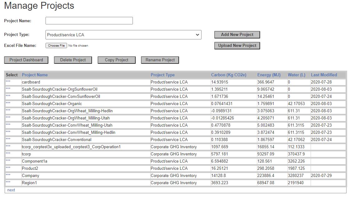
1. Creating and Managing Projects

Click on Manage Projects at the top to see a summary list of all your projects along with the three life-cycle impact assessment metrics that CarbonScope tracks: Carbon or GHG emissions in Kg of CO2e, energy consumed (primary energy combusted + feedstock energy) in MJ and water consumed in liters . Here you can add new LCA or GHG inventory projects, as well as delete, copy or rename them. Select an existing project in your account by clicking on the *** in the first column. You can also upload a project that was previously saved into an Excel file from the LCA or GHG inventory dashboard. The project summary table can be sorted by clicking on the column headers. The Project Dashboard button will take you to the LCA or GHG inventory dashboard for the selected project.

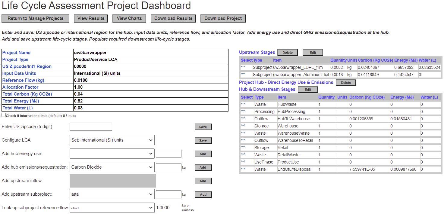
2. LCA Project Dashboard

The life cycle assessment (LCA) project dashboard defines the “hub” or the main/final manufacturing or assembly location for a product. Enter a US zip code or select a country for the hub – this ensures that the electric grid emissions will match the actual location of the hub. The default is US average grid emissions.

Configure the LCA model by setting the input data units (international or US units), the reference flow (the default value is 1; for products, this can be the final weight of the product as delivered or consumed, in kg; it can also be a unitless number if the product or service delivered cannot be measured in kg), and an allocation factor (the default value is 1; set this to a different value between 0 and 1 if there are co-products to indicate the fraction of the life-cycle environmental burdens that should be allocated to the current product). Note that the allocation factor only changes the final carbon/energy/water results, but none of the other tables or data.

Select and add quantities of the various forms of energy used in the hub (electricity, natural gas, propane, heating oil, diesel or gasoline), as well as any direct GHG emissions or sequestration (carbon dioxide, methane or nitrous oxide).

The LCA project comes predefined with one “inflow” stage upstream and ten distinct downstream stages for modeling a full product/service life cycle (more on the details of these stage models in a later section). These predefined stages provide a convenient template for modeling a product/service life cycle. Additional upstream stages can be added as needed using the buttons on the bottom left. These additional upstream stages can be inflows or subprojects. Note that all upstream stages feed directly into the hub, whereas the downstream stages are sequential in the order listed. The predefined downstream stages cannot be deleted, nor can additional downstream stages be added. Depending on the system boundary, you might decide to populate only some of the downstream stages with data. For a typical cradle-to-gate system boundary, only the upstream stages and the hub would be required.

A subproject is a previously defined LCA project in its own right that models the life cycle of a specific material, component or assembly used in the current project. While inflows map incoming materials directly to cradle-to-gate data items in the life-cycle inventory (LCI) database, subprojects can model the life cycles of incoming materials in as much detail as needed. Subprojects can be recursively defined for modeling complex material flows.

The buttons at the top of the dashboard can be used to view results as tables or charts, and download all tables into an Excel file. The entire project model can also be downloaded into an Excel file, which can then be uploaded into a new project by any other CarbonScope user that you share the Excel file with.

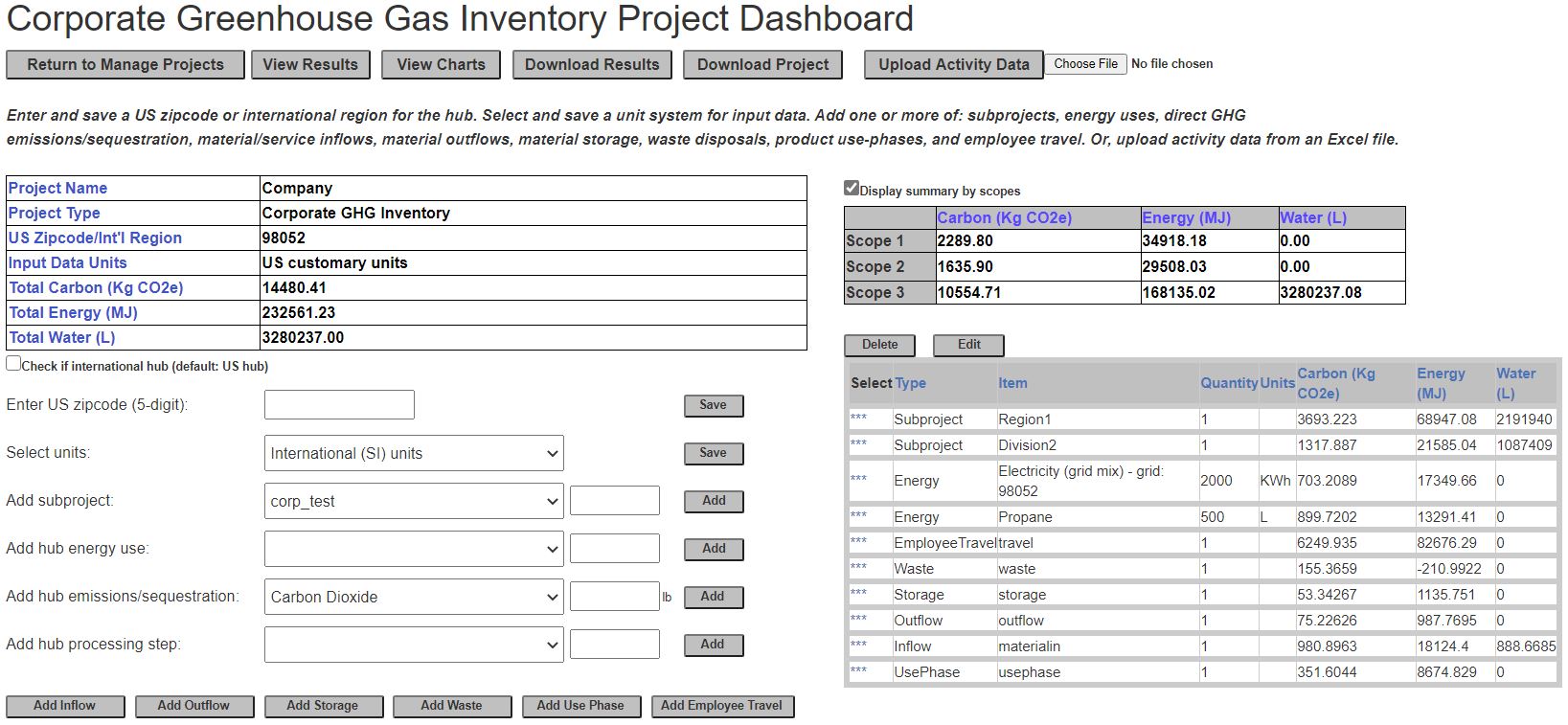
3. GHG Inventory Project Dashboard

The greenhouse gas (GHG) inventory project dashboard defines the “hub” or the primary location (such as the headquarters) of a company or organization. Enter a US zip code or select a country for the hub – this ensures that the electric grid emissions will match the actual location of the hub. The default is US average grid emissions. Then select the input data units as either international or US.

Select and add quantities of the various forms of energy used in the hub (electricity, natural gas, propane, heating oil, diesel or gasoline), as well as any direct GHG emissions or sequestration (carbon dioxide, methane or nitrous oxide). These energy uses, emissions and sequestration will all go into scopes 1 and 2, except for upstream activities such as fuel extraction and processing which will automatically be classified as scope 3.

Use the buttons at the bottom to define one or more “stage models” to define activities that occur outside the direct control of the organization, including upstream and downstream activities. These activities include: inflows of materials or services, outflows of materials/products, storage in a warehouse or retail location, waste disposal, product use phase, and employee travel. More on the details of these stage models in a later section.

There is no limit to the number of stage models within a GHG inventory project. In addition, subprojects can be used to conveniently model distinct departments, divisions or subsidiaries of a company or organization. A subproject is a previously defined GHG inventory project in its own right that models the operation of a clearly defined part of the organization, which in turn can have other subprojects to define smaller entities within.

The buttons at the top of the dashboard can be used to view results as tables or charts, and download all tables into an Excel file. The entire project model can also be downloaded into an Excel file, which can then be uploaded into a new project by any other CarbonScope user that you share the Excel file with.

In addition, activity data for the inventory can be uploaded conveniently from a spreadsheet by selecting an Excel file and clicking the "Upload Activity Data" button. This uses a hybrid methodology as explained in our blog post "Corporate GHG inventories made simple".

4. Stage Models

Stage models are common to both LCA and GHG inventory projects. They represent basic types of activities that occur in an organization or in the life cycle of a product/service. There are six different types of stage models as described below. A project can have one or more instances of each of these, but with these restrictions: LCA projects predefine the downstream stages as indicated above, and employee travel can only be used in GHG inventory projects.

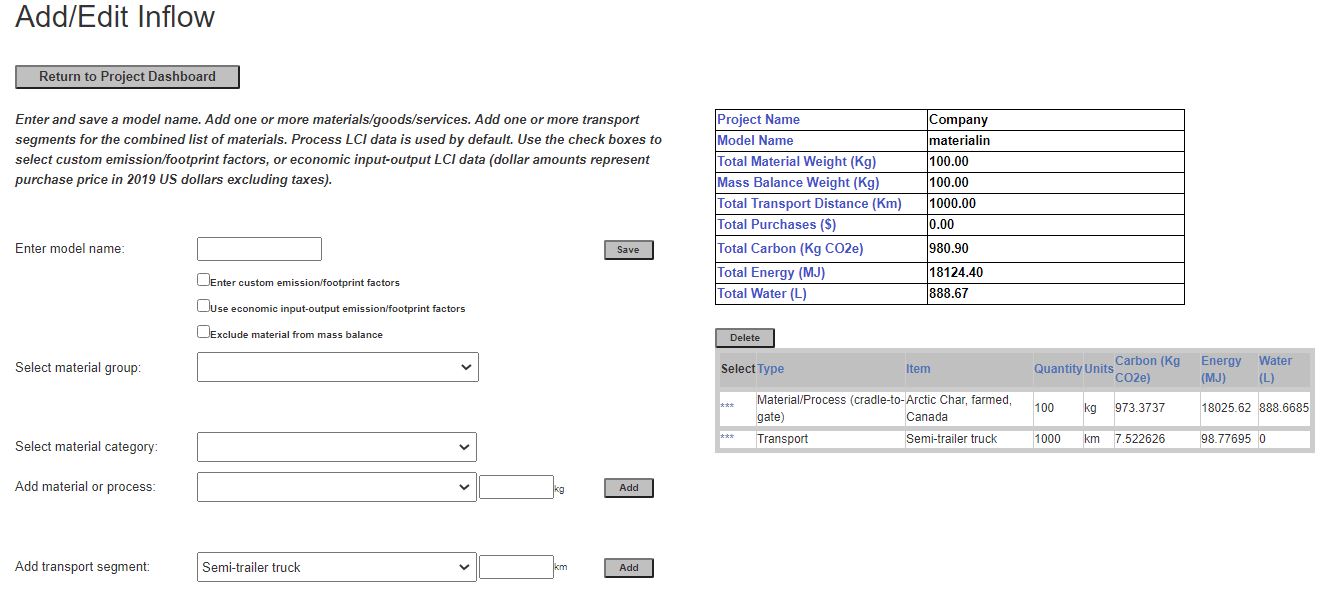
4.1 Inflow

An inflow model is a cradle-to-gate representation of the materials/products or services purchased from other companies. Enter and save a model name before adding any data. By default, the dropdown menus provide conventional process LCI data for cradle-to-gate modeling of materials. Add one or more materials by weight, and then add one or more transport segments for transporting the materials to the hub. An inflow can model multiple materials that are all sourced from the same location and transported using the same transport modes. Use multiple inflow models for materials sourced from different locations or tranpsorted using different modes. If you have custom process LCI data for specific materials, you can check “Enter custom emission/footprint factors” and then add your custom data to the inflow model. For LCA projects, you have the option of excluding specific materials from the mass balance check -- this is used typically for materials that do not go into the final product directly but are consumed as supplies during production.

The alternative to process LCI is environmentally-extended economic input-output LCI data. You can select from this part of the LCI database by checking the “Use economic input-output emission/footprint factors” and then choose goods/services using dollar amounts spent. Dollar amounts represent purchase prices in 2019 US dollars excluding taxes. You will also need to select the most likely supply-chain configuration for each good purchased.

 

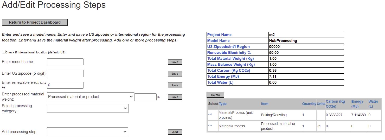
4.2 Processing

A processing model is a unit process representation of one or more pre-defined processing steps associated with the manufacture. This may be related to food processing, fabric production, plastics manufacture, metal fabrication, etc. After defining the model name, simply specify the weight of the material or product and then add as many processing steps as needed, as an alternative to specifying energy consumption directly in the hub. For LCA projects, the material weight will be subject to a mass-balance check against the materials entering the system and any waste generated prior to (i.e., upstream of) the processing model. Enter a US zip code or international location in order to calculate the correct electric grid emissions (the default is US average grid emissions).

 

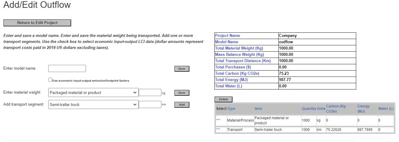
4.3 Outflow

An outflow model represents the transport of finished products from the hub to a downstream location such as a warehouse. After defining the model name, simply specify the weight of the material or product and the transport segments used. For LCA projects, this weight will be subject to a mass-balance check against the materials entering the system and any waste generated prior to (i.e., upstream of) the outflow model. As with inflows, transport can be modeled using dollar amounts spent (2019 US dollars excluding taxes) by checking “Use economic input-output emission/footprint factors”.

 

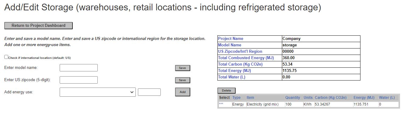
4.4 Storage

A storage model represents warehouses and retail locations. Enter a US zip code or international location in order to calculate the correct electric grid emissions (the default is US average grid emissions). Then add one or more energy items consumed at the storage location for the specific quantity of materials flowing through it.

 

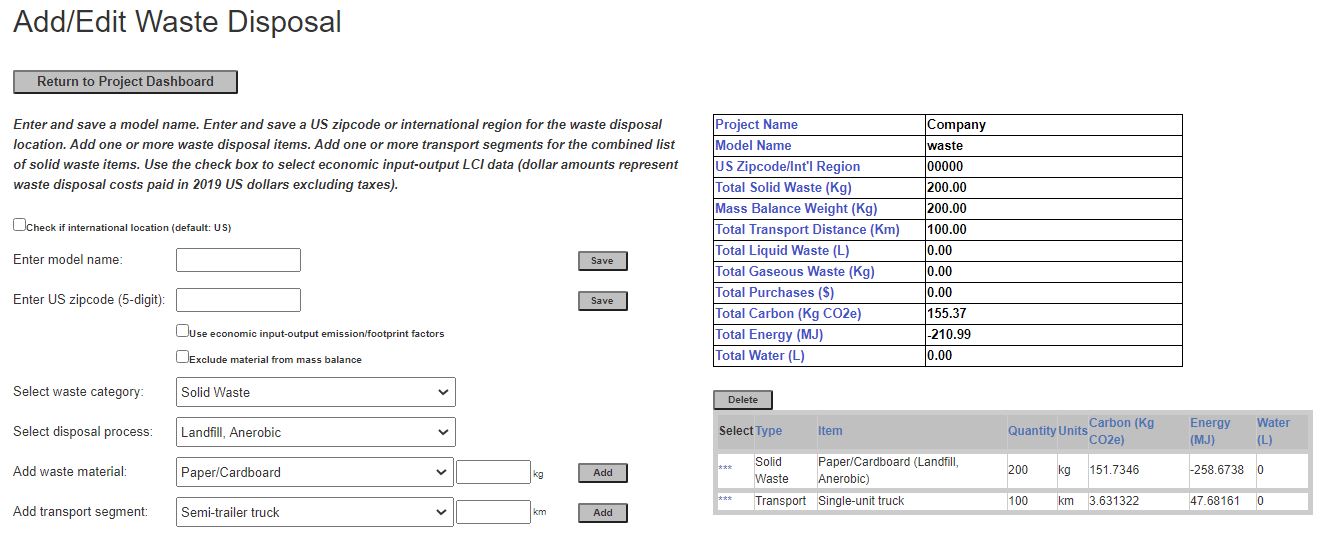
4.5 Waste Disposal

A waste disposal model represents the waste generated at various points in an LCA project or at various locations in a GHG inventory project. Enter a US zip code or international location in order to calculate the correct electric grid emissions for wastewater treatment (the default is US average grid emissions). Use the dropdown menu to select solid, liquid or gaseous waste, the disposal process and the type of material disposed. Add transport segments for solid waste. As with inflows, waste material can be exclued from mass-balance checks in LCA projects. As with inflows and outflows, economic input-output modeling can be used by selecting the checkbox and entering dollar amounts spent on waste disposal.

 

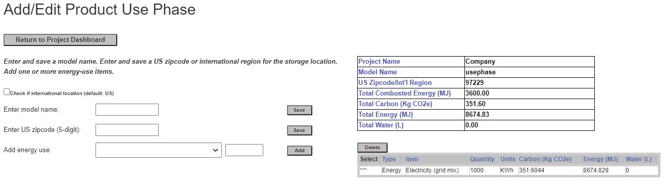
4.6 Use Phase

A use phase model represents the energy consumed during the use of final product in an LCA project or all of the products manufactured by the company in a GHG inventory project. Enter a US zip code or international location in order to calculate the correct electric grid emissions (the default is US average grid emissions). Then add one or more energy items consumed in the product use phase.

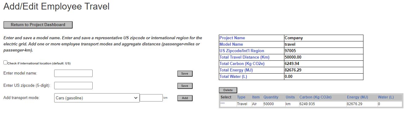
4.7 Employee Travel

An employee travel model captures the impact of employee business travel and commuting. Enter a typical US zip code or international location in order to calculate the best possible electric grid emissions for electric vehicles (the default is US average grid emissions). Then add one or more passenger transport modes along with miles or km traveled by all of the employees combined. For employees in different locations, use multiple employee travel models.

5. Results

The results of an LCA or a GHG inventory can be viewed as tables or charts and downloaded into an Excel file by clicking the appropriate buttons at the top of the LCA or GHG inventory project dashboard. The Excel file includes all the tables mentioned in sections 5.1-5.3.

  

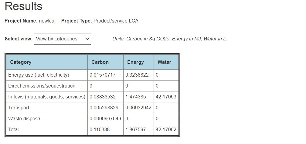
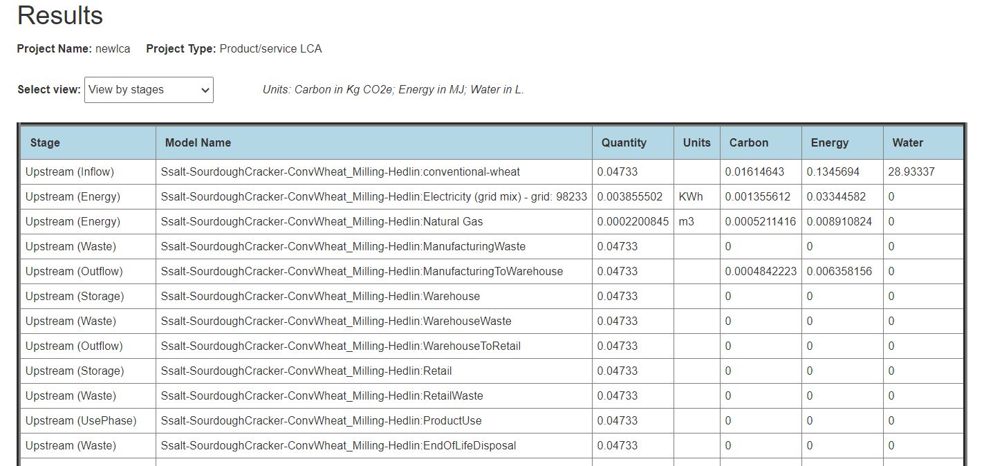
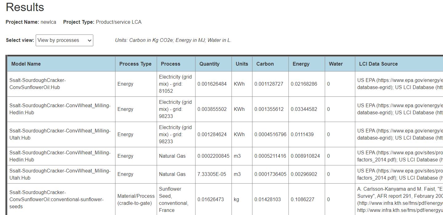
5.1 View results as tables

Available table views include: results by categories, results by stages, results by processes, results by scopes 1-3, and comparison to a baseline project. Sample tables are illustrated below.

 

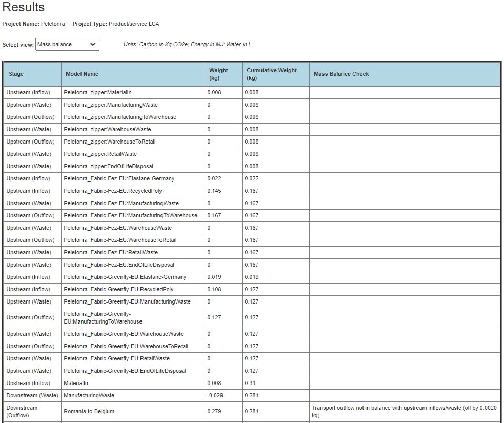
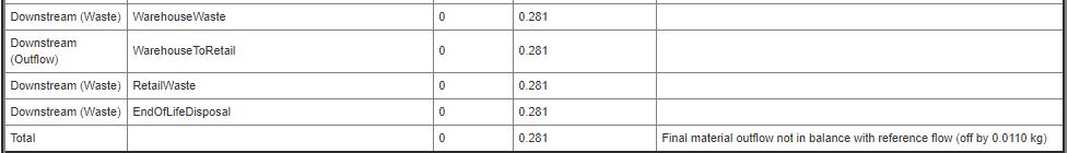
5.2 Mass balance check

For LCA projects, a mass balance check is available in a table format as illustrated below. The cumulative weight of the materials flowing through the product system is tracked through all the stages, and then checked against user-defined transport weights in outflows and the reference flow. The example below shows a mass balance check failing at two points: at an outflow where the weight of material transported does not match the net (inflow minus waste) material upstream, and at the end where the final weight of product delivered does not match the reference flow. The reference flow is used in the mass-balance check only if it is defined as a weight in kg.

 

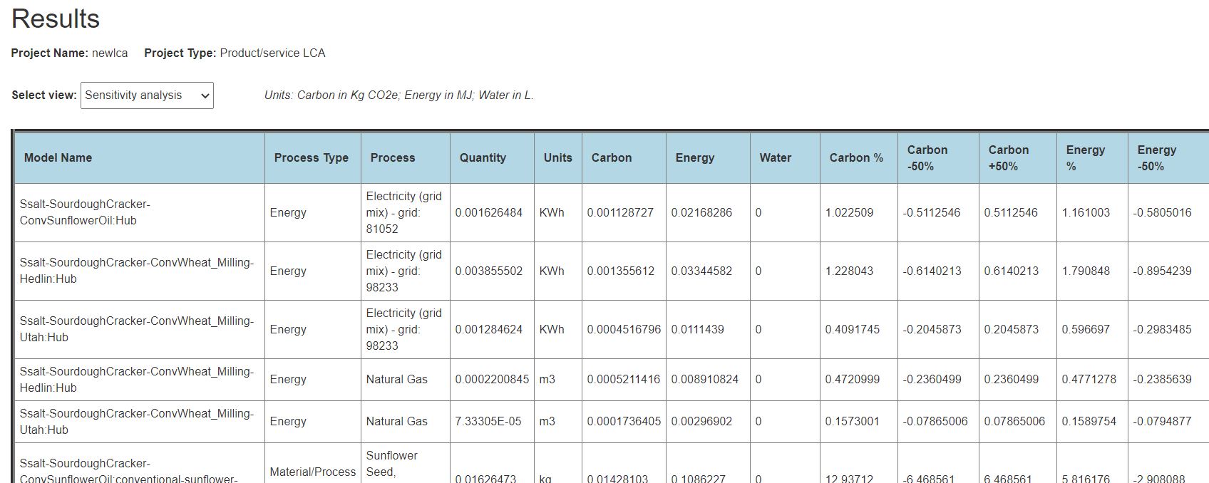
5.3 Sensitivity analysis

A standard way of examining the robustness of a modeling exercise is through a sensitivity analysis of the model parameters. Both LCA and GHG inventory projects can use the sensitivity analysis table to identify processes that contribute most to the final carbon/energy/water impacts and therefore require the most accuracy in both the activity data collected from the production/operation and the emission/footprint factors that CarbonScope takes from the LCI database. The table shows the percentage of the total carbon/energy/water impacts contributed by each process, as well as how much those totals change when the contribution of a particular process changes by +50% and -50%. Processes with low sensitivities may be able to use approximate or placeholder data, while processes with high sensitivities should be modeled with care.

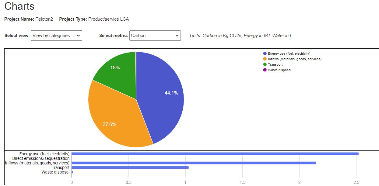
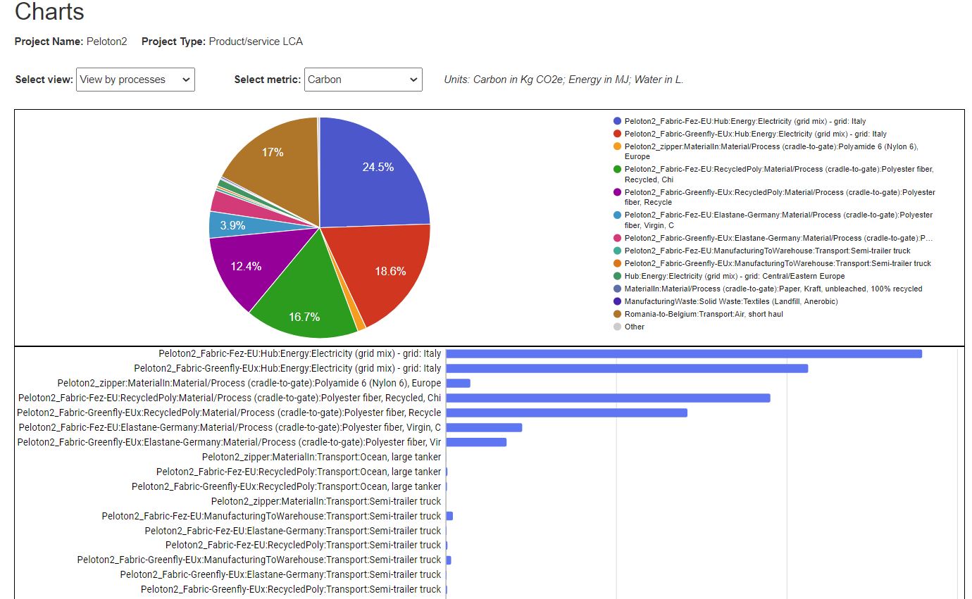
5.4 Viewing results as charts

Available chart views include: results by categories, results by stages, results by processes, results by scopes, and comparison to a baseline project. Sample charts are illustrated below.

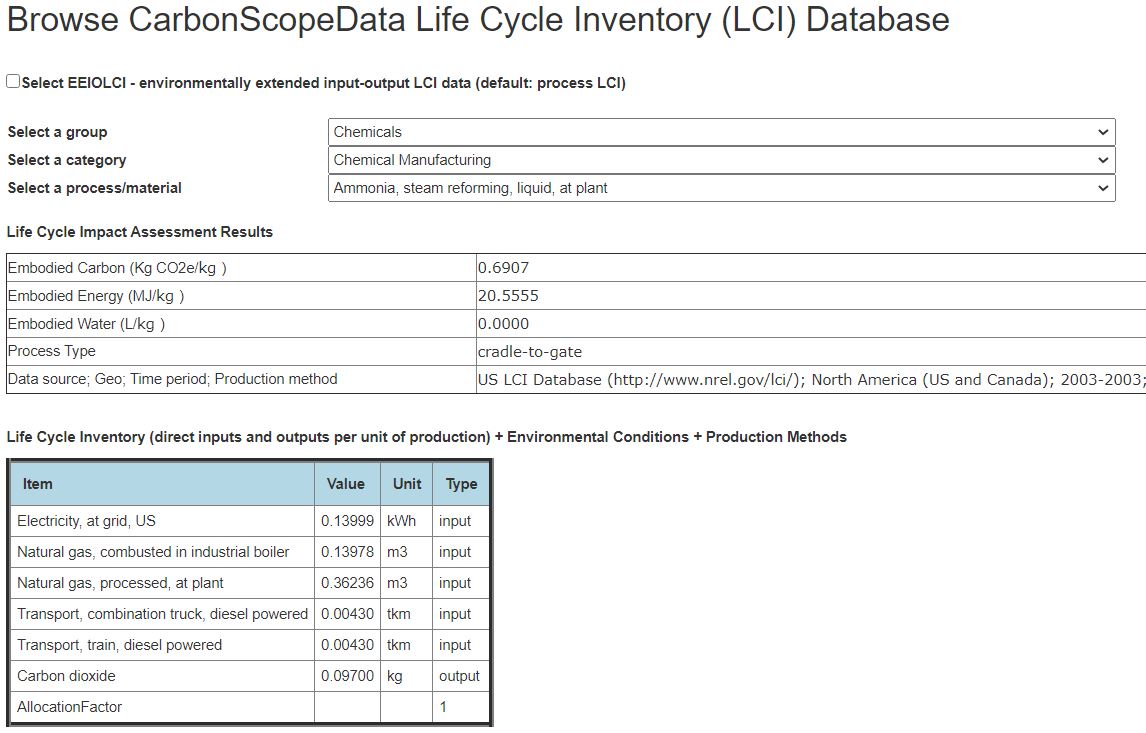
6. Browse/Search LCI Database

Click on LCI Database at the top to browse or search the CarbonScopeData LCI database directly. This is useful if you are just looking for life-cycle inventory data or life-cycle impact assessment results for specific materials, processes or industry sectors. Both the process LCI and the environmentally extended input-output LCI data sets can be accessed.